Classical Mechanics

The Foucault Pendulum

How the Coriolis force produces the slow precession of a pendulum's oscillation plane.

This essay derives the motion of the Foucault pendulum from the equations of motion near Earth's surface. It develops the constrained dynamics, linearizes the pendulum equations, identifies the Coriolis-induced splitting of the circular normal modes, and obtains the precession of the oscillation direction.

Prerequisites

Motion on the Rotating Earth
Dynamics in Rotating Reference Frames
Introductory classical mechanics

Pendulum constraint
Linearized motion
Coriolis coupling
Circular normal modes
Frequency splitting
Precession of the oscillation plane

I. Introduction
II. The Foucault Pendulum
1. Introducing the Pendulum Constraint
2. Gravity Only Case
3. Linearized Equations
4. Solution of the Equations of Motion
5. Precession of the Oscillation Direction

I. Introduction

The equations needed below are obtained in the preceding essay Motion on the Rotating Earth by linearizing the equations of motion near a point on the Earth's surface. Defining dimensional variables of length as

x = ρ_{0} ϕ y = ρ_{0} sin (ϕ_{0}) θ z = ρ

and defining a local coordinate system as

e_{z} = e_{ρ_{0}} e_{y} = e_{θ_{0}} e_{x} = e_{ϕ_{0}}

the linearized equations of motion are

Earth:Local Cartesian Equations

\overset{z}{¨} \overset{x}{¨} \overset{y}{¨} = - g + ω^{2} ρ_{0} sin^{2} ϕ_{0} + ω^{2} sin^{2} ϕ_{0} z + ω^{2} sin (2 ϕ_{0}) x + 2 ω sin ϕ_{0} \overset{y}{˙}, = \frac{1}{2} ω^{2} ρ_{0} sin (2 ϕ_{0}) + \frac{1}{2} ω^{2} sin (2 ϕ_{0}) z + ω^{2} cos (2 ϕ_{0}) x + 2 ω cos ϕ_{0} \overset{y}{˙}, = - 2 ω sin ϕ_{0} \overset{z}{˙} - 2 ω cos ϕ_{0} \overset{x}{˙} .

II. The Foucault Pendulum

In this section, we derive the equations of motion of the Foucault pendulum by applying several simplifying assumptions. The Foucault pendulum is one of the most elegant experiments demonstrating the rotation of the Earth. It consists of a heavy mass

m

suspended by a long wire or rigid rod of length

l

, free to oscillate in any vertical plane. As the pendulum oscillates, the plane of motion slowly rotates with respect to the Earth due to the Coriolis force.

Before proceeding, it is useful to estimate the relative magnitude of the terms appearing in the equations of motion. The angular velocity of the Earth is

ω = \frac{2 π}{T _{sid}} = \frac{2 π}{86 164 s} \approx 7.2921 \times 1 0^{- 5} s^{- 1},

where

T_{sid}

denotes one sidereal day. For a typical Foucault pendulum with length between

15 m

and

30 m

, the natural angular frequency is

ω_{0} = \frac{g}{l} \approx 0.57 - 0.81 s^{- 1},

and therefore

\frac{ω}{ω _{0}} = ω \frac{l}{g} \sim 1 0^{- 4} .

The Coriolis terms in the equations of motion are proportional to

ω

, whereas the centrifugal corrections are proportional to

ω^{2}

. We shall therefore retain only terms up to first order in the Earth's angular velocity, neglecting all terms of order

ω^{2} .

Equation local cartesian equations consequently reduces to

Earth:First Order Local Equations

\overset{x}{¨} \overset{y}{¨} \overset{z}{¨} = 2 ω cos (ϕ_{0}) \overset{y}{˙}, = - 2 ω sin (ϕ_{0}) \overset{z}{˙} - 2 ω cos (ϕ_{0}) \overset{x}{˙}, = - g + 2 ω sin (ϕ_{0}) \overset{y}{˙} .

These equations describe the motion of a particle subjected only to gravity and the Coriolis force. The constraint force exerted by the pendulum wire will be introduced in the next section. Introducing the position vector

p = x e_{x} + y e_{y} + z e_{z},

the Coriolis force can be written in vector form as

F_{cor} = - 2 m ω \times \dot{p},

where the Earth's angular velocity expressed in the local Cartesian basis introduced in the previous section is

ω = ω (- sin (ϕ_{0}) e_{x} + cos (ϕ_{0}) e_{z}) .

Explicitly,

F_{cor} = m 2 ω cos (ϕ_{0}) \overset{y}{˙} - 2 ω sin (ϕ_{0}) \overset{z}{˙} - 2 ω cos (ϕ_{0}) \overset{x}{˙} 2 ω sin (ϕ_{0}) \overset{y}{˙} .

The Coriolis force admits the generalized potential

V_{cor} = - m ⟨ ω \times p ∣ \dot{p} ⟩,

which, in local Cartesian coordinates, becomes

V_{cor} = mω (y cos (ϕ_{0}) \overset{x}{˙} - (sin (ϕ_{0}) z + cos (ϕ_{0}) x) \overset{y}{˙} + sin (ϕ_{0}) y \overset{z}{˙}) .

Including gravity, the corresponding Lagrangian is therefore

L = \frac{1}{2} m (\overset{x}{˙}^{2} + \overset{y}{˙}^{2} + \overset{z}{˙}^{2}) - mω [y (cos (ϕ_{0}) \overset{x}{˙} + sin (ϕ_{0}) \overset{z}{˙}) - \overset{y}{˙} (cos (ϕ_{0}) x + sin (ϕ_{0}) z)] - m g z .

1. Introducing the Pendulum Constraint

The equations derived so far describe the motion of a free particle in the rotating frame of the Earth. To obtain the equations of motion of the Foucault pendulum, we must now introduce the geometric constraint imposed by the rigid wire. One possible approach would be to introduce spherical coordinates centred at the point of suspension. In these coordinates the pendulum constraint is automatically satisfied by fixing the radial coordinate equal to the length of the pendulum. However, this choice is not particularly convenient. The equilibrium configuration of the pendulum corresponds to the bob hanging vertically below the point of suspension, which is precisely the pole of the spherical coordinate system. At this point the azimuthal angle becomes undefined, making spherical coordinates poorly suited for the linearization that follows. Instead, we retain the local Cartesian coordinates

(x, y, z)

introduced in the previous section. We choose the origin of this coordinate system to coincide with the equilibrium position of the pendulum bob. Consequently, the point of suspension has coordinates

(0, 0, l),

where

l

denotes the length of the pendulum.

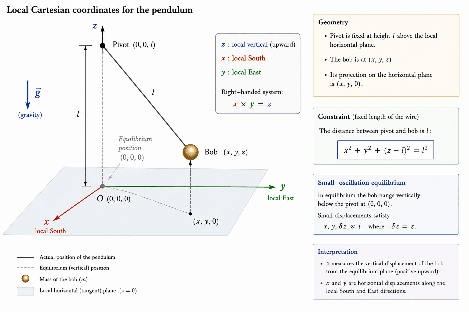
Local Cartesian coordinates of the pendulum.

The motion of the bob is therefore constrained to remain on the sphere of radius

l

centred at the point of suspension. The corresponding holonomic constraint is

g (x, y, z) = x^{2} + y^{2} + (z - l)^{2} - l^{2} = 0.

We introduce a Lagrange multiplier

λ (t)

and define the augmented Lagrangian

F = L - λ g .

The equations of motion for the generalized coordinates

q_{i} = (x, y, z)

are

\frac{d}{d t} (\frac{\partial F}{\partial q ˙ _{i}}) - \frac{\partial F}{\partial q _{i}} = 0.

These equations are supplemented by the constraint

g (x, y, z) = 0.

Applying the Euler--Lagrange equations to the augmented Lagrangian immediately yields

Eq:Foucault Constrained

⎩ ⎨ ⎧ m \overset{x}{¨} - 2 mω cos (ϕ_{0}) \overset{y}{˙} - 2 λ x m \overset{y}{¨} + 2 mω (cos (ϕ_{0}) \overset{x}{˙} + sin (ϕ_{0}) \overset{z}{˙}) - 2 λ y m \overset{z}{¨} - 2 mω sin (ϕ_{0}) \overset{y}{˙} + m g - 2 λ (z - l) x^{2} + y^{2} + (z - l)^{2} = 0, = 0, = 0, = l^{2} .

2. Gravity Only Case

Before considering the complete system, it is useful to make a short detour and examine the pendulum in the absence of the Earth's rotation. This simpler case will clarify both the role of the Lagrange multiplier and the linearization of the constraint around the equilibrium configuration. Setting

ω = 0

, the constrained equations of motion become

Eq:Pendulum Gravity Constrained

⎩ ⎨ ⎧ m \overset{x}{¨} - 2 λ x m \overset{y}{¨} - 2 λ y m \overset{z}{¨} + m g - 2 λ (z - l) x^{2} + y^{2} + (z - l)^{2} = 0, = 0, = 0, = l^{2} .

The equilibrium position of the bob is

x = y = z = 0.

We consider small oscillations around this configuration and write

z = δ z, ∣ δ z ∣ ≪ l .

Expanding the constraint gives

x^{2} + y^{2} + δ z^{2} - 2 l δ z = 0.

Since

δ z ≪ l

, the term

z^{2}

can be neglected, and the constraint reduces to

Eq:Pendulum Linearized Constraint

x^{2} + y^{2} = 2 l δ z .

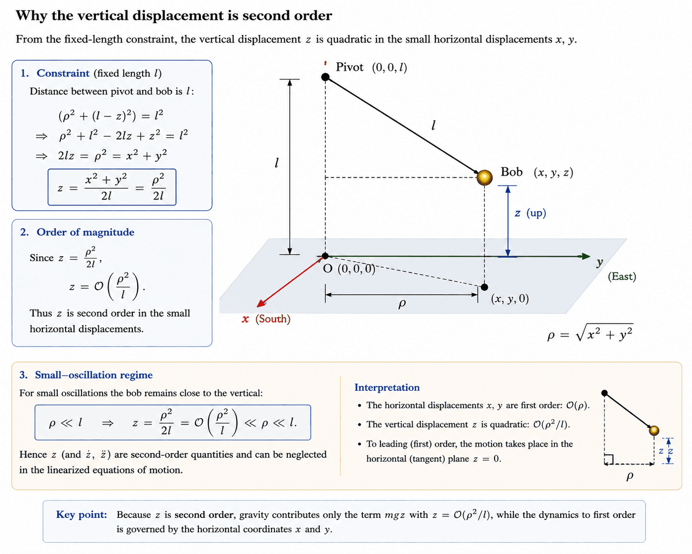
Why the vertical displacement is second order.

This relation shows that, if

x

and

y

are treated as first-order displacements, then

δ z

is a second-order quantity:

δ z = \frac{x ^{2} + y ^{2}}{2 l} .

We now eliminate the Lagrange multiplier from the equations for

y

and

z

. Multiplying the equation for

y

z - l

, multiplying the equation for

z

y

, and subtracting the latter from the former, we obtain

m \overset{y}{¨} (z - l) - m \overset{z}{¨} y - m g y = 0.

Equivalently,

- m l \overset{y}{¨} + m z \overset{y}{¨} - m \overset{z}{¨} y - m g y = 0.

The displacement

z

and its derivatives are of second order in the horizontal oscillation amplitude. Consequently, the terms

z \overset{y}{¨}

and

\overset{z}{¨} y

are of higher order and can be neglected in the linear approximation. We are therefore left with

- m l \overset{y}{¨} - m g y = 0,

Eq:Pendulum Y Equation

\overset{y}{¨} + \frac{g}{l} y = 0.

Repeating the same procedure with the equations for

x

and

z

gives

Eq:Pendulum X Equation

\overset{x}{¨} + \frac{g}{l} x = 0.

Thus, to first order in the horizontal displacements, the two components of the motion satisfy the well known independent harmonic-oscillator equations of the pendulum under gravity

Eq:Ordinary Pendulum Linearized

⎩ ⎨ ⎧ \overset{x}{¨} + \frac{g}{l} x \overset{y}{¨} + \frac{g}{l} y = 0, = 0.

The corresponding natural angular frequency is

ω_{0} = \frac{g}{l} .

3. Linearized Equations

We now return to the complete equations of motion, including the Coriolis force, and repeat the same procedure used in the gravity-only case. We begin with the equations for

y

and

z

m \overset{y}{¨} + 2 mω (cos ϕ_{0} \overset{x}{˙} + sin ϕ_{0} \overset{z}{˙}) - 2 λ y = 0,

and

m \overset{z}{¨} - 2 mω sin ϕ_{0} \overset{y}{˙} + m g - 2 λ (z - l) = 0.

Multiplying the first equation by

z - l

, the second by

y

, and subtracting the latter from the former, we eliminate the Lagrange multiplier and obtain

m \overset{y}{¨} (z - l) + 2 mω (cos ϕ_{0} \overset{x}{˙} + sin ϕ_{0} \overset{z}{˙}) (z - l) - m \overset{z}{¨} y + 2 mω sin ϕ_{0} \overset{y}{˙} y - m g y = 0.

As in the gravity-only case, we consider small vertical displacements around the equilibrium position. We therefore use

z - l ≃ - l

and neglect

z

\overset{z}{˙}

, and

\overset{z}{¨}

, since they are of higher order in the horizontal oscillation amplitude. The equation consequently reduces to

- m l \overset{y}{¨} - 2 mω l cos ϕ_{0} \overset{x}{˙} + 2 mω sin ϕ_{0} y \overset{y}{˙} - m g y = 0.

Dividing by

- m l

, we obtain

Eq:Foucault Y Partially Linearized

\overset{y}{¨} + 2 ω cos ϕ_{0} \overset{x}{˙} - \frac{2 ω}{l} sin ϕ_{0} y \overset{y}{˙} + \frac{g}{l} y = 0.

We proceed in the same way with the equations for

x

and

z

. Multiplying the equation for

x

z - l

, the equation for

z

x

, and subtracting, gives

m \overset{x}{¨} (z - l) - 2 mω cos ϕ_{0} \overset{y}{˙} (z - l) - m \overset{z}{¨} x + 2 mω sin ϕ_{0} x \overset{y}{˙} - m g x = 0.

Using again

z - l ≃ - l

and neglecting

\overset{z}{¨}

, we find

- m l \overset{x}{¨} + 2 mω l cos ϕ_{0} \overset{y}{˙} + 2 mω sin ϕ_{0} x \overset{y}{˙} - m g x = 0,

and therefore

Eq:Foucault X Partially Linearized

\overset{x}{¨} - 2 ω cos ϕ_{0} \overset{y}{˙} - \frac{2 ω}{l} sin ϕ_{0} x \overset{y}{˙} + \frac{g}{l} x = 0.

The constraint must still be imposed. Its leading nonvanishing approximation around the equilibrium position is

x^{2} + y^{2} + z^{2} - 2 l z = 0 ⟹ 2 l z = x^{2} + y^{2},

where

z^{2}

has been neglected with respect to

2 l z

. We therefore obtain the partially linearized constrained system

Eq:Foucault Partially Linearized System

⎩ ⎨ ⎧ \overset{y}{¨} + 2 ω cos ϕ_{0} \overset{x}{˙} - \frac{2 ω}{l} sin ϕ_{0} y \overset{y}{˙} + \frac{g}{l} y \overset{x}{¨} - 2 ω cos ϕ_{0} \overset{y}{˙} - \frac{2 ω}{l} sin ϕ_{0} x \overset{y}{˙} + \frac{g}{l} x 2 l z = 0, = 0, = x^{2} + y^{2} .

We now complete the linearization of the equations of motion. Let the horizontal displacements

x

and

y

be small compared with the length of the pendulum,

∣ x ∣ ≪ l, ∣ y ∣ ≪ l .

The velocities

\overset{x}{˙}

and

\overset{y}{˙}

are of the same perturbative order as the corresponding displacements. Consequently, the mixed terms

x \overset{y}{˙}, y \overset{y}{˙}

are of second order in the oscillation amplitude and can be neglected in the linear approximation. The equations of motion then reduce to

Eq:Foucault Linearized Equations

⎩ ⎨ ⎧ \overset{y}{¨} + 2 ω cos ϕ_{0} \overset{x}{˙} + \frac{g}{l} y \overset{x}{¨} - 2 ω cos ϕ_{0} \overset{y}{˙} + \frac{g}{l} x 2 l z = 0, = 0, = x^{2} + y^{2} .

4. Solution of the Equations of Motion

We transform the second-order system into an equivalent first-order system by introducing the auxiliary variables

u = \overset{x}{˙}, v = \overset{y}{˙} .

The vertical constraint no longer enters explicitly into the horizontal equations of motion and will therefore be omitted in what follows. It can always be recovered afterwards from

2 l z = x^{2} + y^{2} .

Defining

α = 2 ω cos ϕ_{0}, β = \frac{g}{l},

the equations become

⎩ ⎨ ⎧ \overset{x}{˙} \overset{y}{˙} \overset{u}{˙} \overset{v}{˙} = u, = v, = α v - β x, = - α u - β y .

The system can now be written in matrix form as

\frac{d}{d t} x y u v = 00 - β 0 000 - β 100 - α 01 α 0 x y u v .

The general solution of this system is determined by the eigenvalues and eigenvectors of the coefficient matrix. A straightforward calculation shows that the four eigenvalues are

γ_{1, 2} γ_{3, 4} = \pm i ω_{1}, = \pm i ω_{2},

where

ω_{1} ω_{2} = \frac{α ^{2} + 2 β + α α ^{2} + 4 β}{2}, = \frac{α ^{2} + 2 β - α α ^{2} + 4 β}{2} .

The system therefore possesses four distinct eigenvalues corresponding to two independent oscillation frequencies. It is worth observing that, in the absence of the Coriolis force (

α = 0

), the two frequencies become equal,

ω_{1} = ω_{2} = β = \frac{g}{l},

and the eigenvalues become doubly degenerate. The Coriolis force therefore removes this degeneracy, splitting the single natural frequency of the ordinary pendulum into two distinct oscillation frequencies.

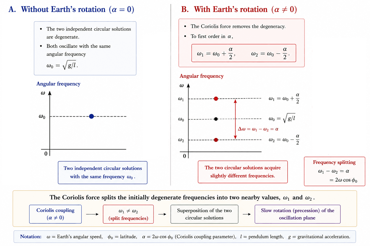
Splitting of the normal-mode frequencies by the Coriolis force.

We now determine the corresponding eigenvectors. Since the procedure is identical for each eigenvalue, we derive only the first one in detail. For the eigenvalue

γ_{1} = i ω_{1},

the eigenvalue equation

(A - γ_{1} I) v_{1} = 0

reads

i ω_{1} 0 β 0 0 i ω_{1} 0 β - 1 0 i ω_{1} α 0 - 1 - α i ω_{1} x y u v = 0000 .

The first two equations immediately give

u = i ω_{1} x, v = i ω_{1} y .

Substituting these expressions into the third equation yields

(β - ω_{1}^{2}) x = i α ω_{1} y,

y = i \frac{ω _{1}^{2} - β}{α ω _{1}} x .

Since eigenvectors are defined up to an arbitrary multiplicative constant, we choose

x = 1.

The corresponding eigenvector is therefore

v_{1} = 1 i \frac{ω _{1}^{2} - β}{α ω _{1}} i ω_{1} \frac{β - ω _{1}^{2}}{α}

For convenience, we introduce the quantities

η_{1} = \frac{ω _{1}^{2} - β}{α ω _{1}}, η_{2} = \frac{ω _{2}^{2} - β}{α ω _{2}} .

The corresponding eigenvectors are

v_{1} = 1 i η_{1} i ω_{1} - ω_{1} η_{1}, v_{3} = 1 i η_{2} i ω_{2} - ω_{2} η_{2},

while the remaining two eigenvectors are simply their complex conjugates,

v_{2} = \overline{v}_{1}, v_{4} = \overline{v}_{3} .

The general solution of the system can therefore be written as

x y u v = c_{1} v_{1} e^{i ω_{1} t} + c_{2} v_{2} e^{- i ω_{1} t} + c_{3} v_{3} e^{i ω_{2} t} + c_{4} v_{4} e^{- i ω_{2} t},

where the constants

c_{1}, c_{2}, c_{3}, c_{4}

are determined by the initial conditions. To illustrate the motion, we consider the pendulum released from rest after a small displacement

d

along the

x

-axis,

x (0) y (0) u (0) v (0) = d 000

This choice is not restrictive. Since the equations of motion are invariant under rotations in the horizontal plane, any other initial displacement can be obtained from this solution by a suitable rotation of the coordinate system. Imposing these initial conditions uniquely determines the coefficients

c_{1}, c_{2}, c_{3}, c_{4}

. After straightforward algebra, the horizontal motion is found to be

x (t) y (t) = \frac{d}{2} [\frac{α}{α ^{2} + 4 β} (cos (ω_{2} t) - cos (ω_{1} t)) + cos (ω_{1} t) + cos (ω_{2} t)], = \frac{d}{α ^{2} + 4 β} [ω_{1} sin (ω_{2} t) - ω_{2} sin (ω_{1} t)] .

The expressions obtained above can be rewritten in a more revealing form, in which the half-sum and half-difference of the two eigenfrequencies appear explicitly. We begin with the expression for

y (t)

y (t) = \frac{d}{α ^{2} + 4 β} [ω_{1} sin (ω_{2} t) - ω_{2} sin (ω_{1} t)] .

The quantity inside the brackets can be rearranged as

ω_{1} sin (ω_{2} t) - ω_{2} sin (ω_{1} t) = \frac{ω _{1} - ω _{2}}{2} [sin (ω_{1} t) + sin (ω_{2} t)] - \frac{ω _{1} + ω _{2}}{2} [sin (ω_{1} t) - sin (ω_{2} t)] .

We now use the sum-to-product identities

sin a + sin b = 2 sin (\frac{a + b}{2}) cos (\frac{a - b}{2}),

and

sin a - sin b = 2 cos (\frac{a + b}{2}) sin (\frac{a - b}{2}) .

It follows that

y (t) = \frac{d}{α ^{2} + 4 β} [(ω_{1} - ω_{2}) cos (\frac{ω _{1} - ω _{2}}{2} t) sin (\frac{ω _{1} + ω _{2}}{2} t) - (ω_{1} + ω_{2}) cos (\frac{ω _{1} + ω _{2}}{2} t) sin (\frac{ω _{1} - ω _{2}}{2} t)] .

We proceed in the same way with

x (t)

x (t) = \frac{d}{2} [\frac{α}{α ^{2} + 4 β} (cos (ω_{2} t) - cos (ω_{1} t)) + cos (ω_{1} t) + cos (ω_{2} t)] .

Using the identities

cos a + cos b = 2 cos (\frac{a + b}{2}) cos (\frac{a - b}{2}),

and

cos b - cos a = 2 sin (\frac{a + b}{2}) sin (\frac{a - b}{2}),

we find

x (t) = d [cos (\frac{ω _{1} - ω _{2}}{2} t) cos (\frac{ω _{1} + ω _{2}}{2} t) + \frac{α}{α ^{2} + 4 β} sin (\frac{ω _{1} - ω _{2}}{2} t) sin (\frac{ω _{1} + ω _{2}}{2} t)] .

The solution can therefore be written in the final form

Eq:Foucault Sum Difference Solution

⎩ ⎨ ⎧ x (t) y (t) = d [cos (\frac{ω _{1} - ω _{2}}{2} t) cos (\frac{ω _{1} + ω _{2}}{2} t) + \frac{α}{α ^{2} + 4 β} sin (\frac{ω _{1} - ω _{2}}{2} t) sin (\frac{ω _{1} + ω _{2}}{2} t)], = \frac{d}{α ^{2} + 4 β} [(ω_{1} - ω_{2}) cos (\frac{ω _{1} - ω _{2}}{2} t) sin (\frac{ω _{1} + ω _{2}}{2} t) - (ω_{1} + ω_{2}) cos (\frac{ω _{1} + ω _{2}}{2} t) sin (\frac{ω _{1} - ω _{2}}{2} t)] .

We now examine the behavior of the two eigenfrequencies when the Coriolis coupling is small. Since

α = 2 ω cos ϕ_{0}

is much smaller than the natural frequency of the pendulum, we expand

ω_{1}

and

ω_{2}

around

α = 0

. At

α = 0

, both frequencies reduce to

ω_{1} (0) = ω_{2} (0) = β .

For the first frequency,

ω_{1} = \frac{α ^{2} + 2 β + α α ^{2} + 4 β}{2},

and its derivative at

α = 0

\frac{d ω _{1}}{d α}_{α = 0} = \frac{1}{2} .

Similarly,

ω_{2} = \frac{α ^{2} + 2 β - α α ^{2} + 4 β}{2},

and

\frac{d ω _{2}}{d α}_{α = 0} = - \frac{1}{2} .

The Taylor expansions to first order in

α

are therefore

ω_{1} ω_{2} = β + \frac{α}{2} + O (α^{2}), = β - \frac{α}{2} + O (α^{2}) .

It follows immediately that

ω_{1} + ω_{2} ω_{1} - ω_{2} = 2 β + O (α^{2}), = α + O (α^{3}) .

Thus, to the required order,

\frac{ω _{1} + ω _{2}}{2} ≃ β, \frac{ω _{1} - ω _{2}}{2} ≃ \frac{α}{2} .

Substituting these expressions into foucault sum difference solution , we obtain

Eq:Foucault Frequency Expanded Solution

⎩ ⎨ ⎧ x (t) y (t) ≃ d [cos (\frac{α}{2} t) cos (β t) + \frac{α}{α ^{2} + 4 β} sin (\frac{α}{2} t) sin (β t)], ≃ \frac{d}{α ^{2} + 4 β} [α cos (\frac{α}{2} t) sin (β t) - 2 β cos (β t) sin (\frac{α}{2} t)] .

We now perform the final simplification. Since

\frac{α}{α ^{2} + 4 β} ≃ \frac{α}{2 β} ≪ 1,

the second term in

x (t)

is a small correction to its leading term and can be neglected. Similarly, in the expression for

y (t)

, the term proportional to

α

is negligible compared with the term proportional to

2 β

. We also use

α^{2} + 4 β ≃ 2 β .

It is important, however, not to expand the functions

cos (\frac{α}{2} t), sin (\frac{α}{2} t),

because their variation occurs over the long time scale associated with the precession of the pendulum. The horizontal motion therefore reduces to

Eq:Foucault Final Solution Alpha Beta

⎩ ⎨ ⎧ x (t) y (t) = d cos (\frac{α}{2} t) cos (β t), = - d sin (\frac{α}{2} t) cos (β t) .

Recalling that

α = 2 ω cos ϕ_{0}, β = \frac{g}{l},

we finally obtain

Eq:Foucault Final Solution

⎩ ⎨ ⎧ x (t) y (t) = d cos (ω cos ϕ_{0} t) cos (\frac{g}{l} t), = - d sin (ω cos ϕ_{0} t) cos (\frac{g}{l} t) .

5. Precession of the Oscillation Direction

The form of the solution admits a particularly simple geometric interpretation. Introducing the rotation matrix

R (ϑ) = (cos ϑ sin ϑ - sin ϑ cos ϑ),

the horizontal motion can be written as

Eq:Foucault Rotating Direction

(x (t) y (t)) = R (- ω cos ϕ_{0} t) (d cos (\frac{g}{l} t) 0) .

The pendulum therefore performs a rapid oscillation with angular frequency

\frac{g}{l},

along the horizontal unit vector

n (t) = cos (ω cos ϕ_{0} t) e_{x} - sin (ω cos ϕ_{0} t) e_{y} .

This direction rotates slowly with angular velocity

- ω cos ϕ_{0} .

Together with the local vertical direction,

n (t)

determines the instantaneous plane of oscillation of the pendulum. It is in this precise sense that the plane of oscillation is said to rotate relative to the Earth. The underlying dynamical mechanism, however, is the splitting of the two circular normal modes by the Coriolis force. In the absence of the Earth's rotation, the two modes have the same frequency. The Coriolis coupling removes this degeneracy, and the gradual accumulation of their relative phase produces the slow precession of the oscillation direction.

The Foucault Pendulum

How the Coriolis force produces the slow precession of a pendulum's oscillation plane.

Prerequisites

Contents

Contents

I. Introduction

II. The Foucault Pendulum

1. Introducing the Pendulum Constraint

2. Gravity Only Case

3. Linearized Equations

4. Solution of the Equations of Motion

5. Precession of the Oscillation Direction