
Classical Mechanics
The Kinematics of Rotations
Orthogonal transformations, finite and infinitesimal rotations, angular velocity, and rotating reference frames.
This essay develops the kinematics of rigid body motion from first principles, emphasizing geometric intuition, careful derivation, and precise notation. Beginning with orthogonal transformations, we construct the mathematical framework required to describe the motion of rigid bodies and rotating reference frames.
Prerequisites
- Linear algebra and matrix transformations
- Vector calculus
- Introductory classical mechanics
Contents
I. Introduction
In this essay we will explore the kinematics of rotations. A more general discussion of the possible motions of a rigid body will be left to a future essay. Here we will cover the following topics:
- •Basic Properties of Orthogonal Transformations: We will review the properties of orthogonal transformations, which preserve distances while leaving the origin fixed and therefore provide the natural mathematical description of rigid rotations.
- •Rotations in Three Dimensions: We will specialize to three-dimensional space and derive the representation of finite rotations about both principal and arbitrary axes.
- •Infinitesimal Rotations: We will then study infinitesimal changes of orientation and show how they can be represented by a vector.
- •Angular Velocity: From infinitesimal rotations we will introduce the angular velocity vector, which describes the instantaneous rate of change of orientation.
- •Transformation of Vectors Between Reference Frames: Using angular velocity, we will derive the relation between the time derivatives of a vector measured in fixed and rotating reference frames, and examine rotations about fixed and time-dependent axes.
II. Orthogonal Transformations
As we highligthed in the introduction, we are interested in understanding the mathematical transformations that leave one point, or a set of point lying on a axis invariant, while keeping the distance between points in space invariant. Such transformations are called Orthogonal transformations.
In this section we will review some basic properties of orthogonal transformations in a vector space over the complex numbers of dimension , which is endowed with a scalar product generalized for complex vectors:
where and are complex vectors in , and denotes the complex conjugate of . The scalar product is positive-defined, which means that it satisfies the following properties:
Although the vector space is defined over , we shall consider only matrices with real coefficients. Consequently, all transformations discussed here are orthogonal rather than unitary. The complex scalar product is introduced only because it provides the natural setting for discussing the eigenvalues and eigenvectors of orthogonal matrices.
- •Definition : Orthogonal transformations are linear transformations that preserve the scalar product, and play a crucial role in the theory of rigid body motion. A linear transformation of onto itself,is orthogonal if it preserves the scalar product between any two vectors.,for all .
- •Symmetry and Inverse: From the properties of matrices and scalar products, we can write the above equation aswhich results in,Kinematics:Orthogonal Conditionwhere is the identity matrix. The inverse of an orthogonal transformation is the transpose of the matrix itself. As a note: if the matrix had complex elements, then the transpose would be replaced by the conjugate transpose :
- •Orthogonality of rows and columns : Considering the row and column vectors and forming the matrix , we can write the above equation aswhich is equivalent to requiring that the rows and the columns vectors are a set of orthonormal vectors. The vectors represent the components of the unit vectors that define the direction of the coordinate axes in the rotated system, relative to the unit vectors of the reference system.
- •Property of eigenvalues : The eigenvector corresponding to the eigenvalue will preserve its length under the orthogonal transformation:which implies that the eigenvalues are complex numbers on the complex unit circle of the form , and they always come in pairs, as is an eigenvalue as well. If is even, then one eigenvalue is either or .
- •Property of eigenvectors : the eigenvectors and corresponding to different eigenvalues and are orthogonal to each other. The proof of this property is straightforward, as we can writewhich can only be true if , as the eigenvalues are complex numbers on the unit circle different from zero.
- •Property of determinant From it follows that,which implies that the determinant of an orthogonal matrix is either or . As we will see in the next section, the former corresponds to proper rotations, while the latter corresponds to improper rotations or reflections.
- •The Othogonal Group The set of orthogonal matrices forms a group under matrix multiplication:
- •Multiplying any two orthogonal matrices and gives again an orthogonal matrix,as .
- •Every orthogonal matrix has an inverse, which is the transposed matrix.
- •The identity element is the identity matrix .
- •The matrix multiplication is associative.
The subset of orthogonal matrices with determinant forms a subgroup of the orthogonal group, called the special orthogonal group and denoted by . This group describes proper rotations. - •Interpretation of orthogonal transformation It is important to note that an orthogonal transformation can be seen in either of two ways:
- •a passive transformation, where the components of the same vector are expressed in different bases;
- •an active transformation, where a vector is actively transformed into a new one in the same reference system.
We will observe that in three dimensions, these two interpretations result in rotations that correspond to inverse rotations.
III. Rotations in Three Dimensions
An orthogonal transformation in three dimensions always possesses one real eigenvalue, equal to either +1 or −1. The remaining two eigenvalues are either the complex-conjugate pair and , or another pair of . The eigenvectors corresponding to the eigenvalue are the vectors that remain unchanged under the transformation, forming the rotation axis. Conversely, the eigenvectors corresponding to the eigenvalue are the vectors that are reflected under the transformation. In physics, we assume that an orthogonal transformation varies continuously with the parameter the rotation angle. This angle typically depends on time and describes the evolution of the rotated reference system relative to the fixed reference frame. When the rotation angle is zero, the reference systems coincide, and the transformation is the identity. Since the eigenvalue associated with the rotation axis cannot change continuously from +1 to −1, we restrict our attention to the connected component of the identity, namely the proper rotations.
1. Rotation Around the Principal Axes
Before deriving the general form of a rotation around any axis, we will consider the rotation around the -axis. In Fig~1 such a rotation is illustrated. The rotation matrix in this case is given by,
where is the rotation angle. The derivation of the matrix is straightforward, as the row vectors are obviously the components of the unit vectors of the rotated system in the reference system. The matrix is orthogonal, as it satisfies the properties of an orthogonal matrix, and it is easy to verify that the determinant is . It is important to emphasize that the matrix represents a passive transformation, where the components of the same vector are expressed in different bases, and the rotated reference system is turned by an angle counterclockwise around the -axis. When is interpreted in an active case, the rotation will be clockwise around the -axis. This can be readily verified by considering the effect of applying to a vector ,
which corresponds to decreasing the polar angle by the angle . If the active rotation in practical applications needs to be counterclockwise, the angle must be negative. The rotation matrix around the -axis is given by,
and the one around the -axis is given by,
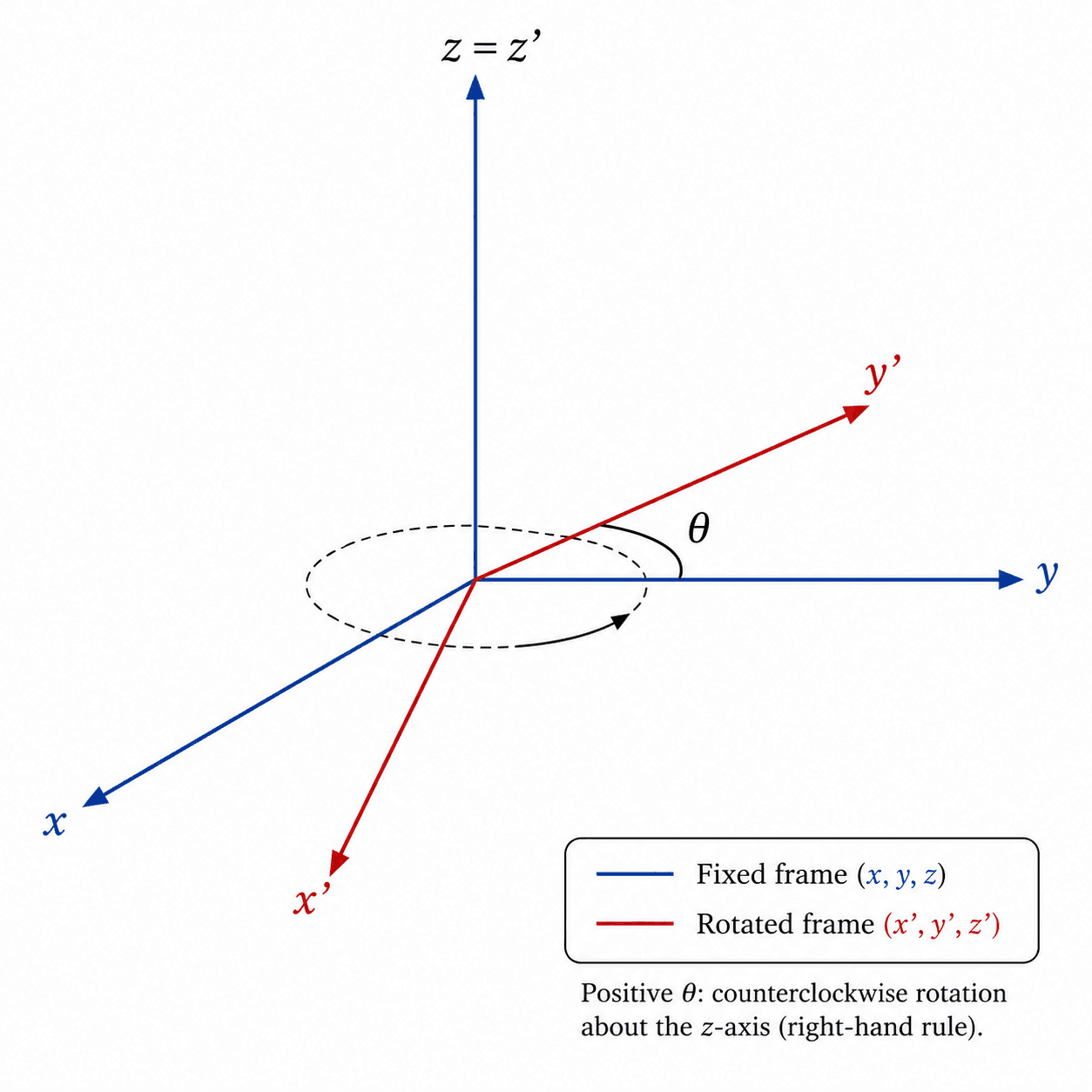
Fig~1: Rotation of an angle around the axis.
2. Rotation Around a General Axis
The formula for a change of coordinates as a result of a rotation around an arbitrary axis defined by the unit vector , with and an angle , is called the Rodrigues formula. While there are numerous well-documented methods to derive this formula available in various resources, we will revisit the derivation process, explaining the steps in detail. Our goal is to find the components of the rotated unit vectors in the reference system as a function of the components of the unit vector and the angle . These components will form the rows of the matrix describing the change of coordinates. A unit vector in the fixed reference system can be decomposed into the component and respectively parallel and perpendicular to :
The component is parallel to the rotation axis, and it will not change under the rotation. The component is perpendicular to the rotation axis, and it will rotate by an angle around the axis , into a new vector . Considering the unit vector along ,
and ,
applying the two-dimensional rotation formula in the plane orthogonal to , we can write the rotated vector as,
as the norm of the vector remains constant. The vector contains only the components of of index different from , as it can be easily verified by the definition of the cross product,
where is the Levi-Civita tensor. The norm of the vector is given by,
The components of the rotated unit vectors with respect to the reference frame are then given by,
The matrix which describes the transformation of a vector's components with respect to a reference system rotated around an axis by an angle , is obtained by evaluating the above equation for each unit vector in the reference system. The components of the vectors with respect to are the rows of the matrix :
Kinematics:Rodrigues Formula
where is the placeholder for a vector. The three terms respectively leave unchanged the component parallel to the rotation axis, rotate the perpendicular component, and generate the component orthogonal to both.
The explicit matrix form of the equation above is,
It is important to emphasize again that the above transformation represents a passive rotation, meaning that the components of the same vector are expressed in different bases. The same matrix, if interpreted as an active transformation, corresponds to the inverse rotation.
IV. Infinitesimal Rotations
1. Definition
In the previous section, we demonstrated that a rotation in three dimensions can be uniquely identified by a unit vector and an angle . It is natural to ask whether the group of orthogonal matrices , is isomorphic to the vector space . This choice is motivated by the fact that every rotation in three dimensions has only three degrees of fredome: the two independent components of the rotation axis, and the rotation angle.
There are several obstacles with defining properly such a isomorphism, as we will soon see, but we will first start by assuming simply that such a an isomorphism exists, between the group with matrix multiplication and the group with the the regular vector addition:
For such an isomorphism to exist, it must be a single-valued function, it must preserve the group operation:
and it has to be one-to-one and surjective. The one-to-one conditions requires that,
Considering two rotations and , we know that rotations do not commute,
However, their images under the mapping are the same,
due to the commutativity of the vector space . Thus, it is evident that such a mapping cannot be one-to-one. Therefore, since the group is not commutative, whereas the group is commutative, no group isomorphism between the two can exist.
We will now introduce the concept of infinitesimal rotations, which are rotations that commute to the first order and allow us to establish an isomorphism the vector space . Let us consider two rotation matrices and such that,
where and are infinitesimal matrices such that products of infinitesimal quantities are neglected. The product of and is,
which is the same as the product of and . Hence, for so-called infinitesimal rotations, the commutativity property holds. For a general infinitesimal rotation , the orthogonal condition implies that the matrix is skew-symmetric, as it satisfies the property
A skew-symmetric matrix has zero diagonal elements, and the off-diagonal elements satisfy the property , and assumes the general form,
A change of coordinates of a vector under an infinitesimal rotation is given by,
as it can be readily verified that,
where and . The infinitesimal vector therefore completely characterizes the infinitesimal rotation. Since infinitesimal rotations commute to first order, the obstruction encountered for finite rotations disappears. It is therefore possible to identify each infinitesimal rotation uniquely with a vector in . We now evaluate the form of the matrix rodrigues formula for a value of the angle that is infinitesimally small. We find that the matrix is given by,
This allows us to identify,
as the infinitesimal rotation matrix, and the vector
as the vector defining the infinitesimal rotation.
2. Similarity Transformation of Infinitesimal Rotations
In the previous section, we have shown that an infinitesimal rotation can be characterized by a vector . We will now show that transforms as a regular vector under a similarity transformation. Let us consider a rotation matrix , where is a skew-symmetric matrix of the form,
The representation of in the coordinate system defined by an orthogonal transformation , is and it has the form,
The matrix is skew-symmetric, as it can be readily verified that,
Given that the matrix is orthogonal, there exist three orthogonal unit vectors , , and :
which define a reference system in the rotated coordinates. The matrix can be written as:
where the vectors are row vectors. The transpose of is readily obtained as:
where the vectors are now the columns of . The product is the matrix with columns:
and, for illustration, the matrix is explicitly written below:
The antisymmetry of the matrix is evident as the diagonal elements are zero:
and the off-diagonal elements are opposite because of the properties of the scalar triple product:
The components of are by definition:
These are simply the independent entries of the transformed skew-symmetric matrix. As the determinant of assumes the values :
depending on the orientation of the vectors in the rotated coordinate system, the equations become:
where we have made use of the property of the scalar triple product. Equation
shows that, under proper orthogonal transformations ( ), the infinitesimal rotation vector transforms exactly as an ordinary vector. Under improper orthogonal transformations ( ), it acquires an additional sign and therefore transforms as an axial vector (or pseudovector).
V. Rate of Change of a Vector
In this section, we will examine how the coordinates of a given vector change over time in two different reference systems: one that is fixed and another that rotates with respect to the fixed one. Although this result is well known, we shall derive it in detail in order to make explicit the meaning of each term appearing in the equations of motion. This will ensure that it is clear which components are being referenced in the general equation of motion. To understand this better, consider a vector in a fixed reference frame and how its components might appear different in a rotating frame. The rotating frame itself can change its orientation with time, adding complexity to the motion of the vector. By carefully deriving the equations, we can delineate the contributions from both the intrinsic change of the vector and the effect of the rotating frame. We will start by defining the vector in the fixed frame and introduce the rotational matrix that relates the rotating frame to the fixed frame. We will then derive the time derivative of the vector in both frames and show how they are connected. Let us consider a time-dependent vector in a fixed reference frame, and its components in a rotating frame . We will assume that the components in the two different reference systems change as per a rotation matrix , which is also time-dependent:
The time derivative of the vector in the rotating frame is given by,
and the time derivative of the matrix at time is formally defined as,
The operator is the composition of two rotations: one from the fixed frame to the rotating frame at time , and the other being the infinitesimal rotation from the rotating frame at time :
and the derivative of the operator is then given by,
To determine the action of this operator, let be an arbitrary vector. Since the infinitesimal matrix acts on the vector after it has already been transformed by , we have
where
is the angular velocity . Since the above relation holds for every vector , we may write
where denotes the placeholder for the vector on which the operator acts. where,
and denotes the placeholder for a vector. is the angular velocity . The final formula for the rate of change of the vector in the rotating frame is then given by the following equivalent equations:
Kinematics:Rotating Frame Derivative
where in the last equation, the distributive property of matrix multiplication for orthogonal matrices regarding the cross product has been utilized. A similar formula can be derived for the rate of change of the vector in the fixed frame, since . Multiplying rotating frame derivative by from the left, we obtain,
Kinematics:Inertial Frame Derivative
1. Poisson Formulas
Let us consider a set of unit vectors fixed in the rotating frame, and let denote the corresponding vectors expressed in the fixed frame. Since the components are constant in the rotating frame, equation rotating frame derivative gives
The quantity
does not denote the ordinary time derivative of the components , which are constant in the rotating reference frame. Instead, throughout this section we define it as the components, expressed in the rotating frame, of the physical time derivative of the basis vector:
With this definition, the previous equation becomes
which is the Poisson formula.
2. Components of the Angular Velocity
Let us consider the Poisson formula for the unit vector ,
Taking the scalar product of both sides with , we obtain, we obtain the component of the angular velocity along the vector:
Similar formulas can be derived for the other components of the angular velocity, and we ultimately obtain:
and in vector form,
Kinematics:Angular Velocity Components
Equation angular velocity components shows that the angular velocity is completely determined by the time evolution of the orthonormal basis attached to the rotating reference frame.
VI. Relevant Examples of Angular Velocity
In this section, we will present several examples of angular velocity in a rotating system. We begin with the case of a rigid body rotating about a fixed axis, and then consider the more general situation in which the axis of rotation also varies with time.
1. Rotation around a Fixed Axis
In this section, we will assume that a rigid body is rotating around a fixed axis by an angle . The time derivative of the rotation matrix from rodrigues formula is given by:
It can be readily verified that:
where the angular velocity in the rotating frame is given by:
Kinematics:Fixed Axis Angular Velocity
Since the rotation axis is invariant under the transformation,
the components of the angular velocity are identical in both the fixed and rotating reference frames.
2. Rotation around a Rotating Axis
The formula for the angular velocity when the axis of rotation is also changing in time can be derived following the same steps as in the previous example. The derivation is algebraically involved, so we present the final result for the angular velocity in the rotating frame:
Kinematics:Moving Axis Angular Velocity
The last term represents the contribution due to the variation of the rotation angle, whereas the first two terms arise from the time dependence of the rotation axis.
The formula above can be verified using symbolic computation software. It is convenient to express in polar coordinates, which automatically enforces the constraint
ensuring that at all times.
The kinematical relations derived in this chapter provide the foundation for the study of dynamics in rotating reference frames. In the next chapter, we will derive the fictitious forces that arise in non-inertial systems, including the centrifugal and Coriolis forces, and apply these results to the motion of bodies on the rotating Earth.